Part 1: Fun with Filters

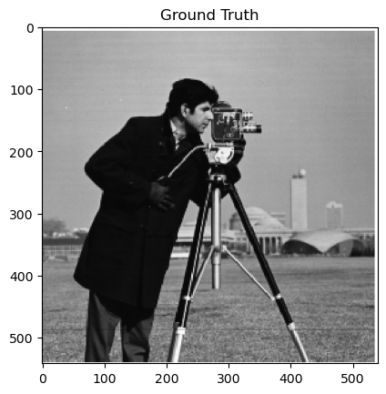
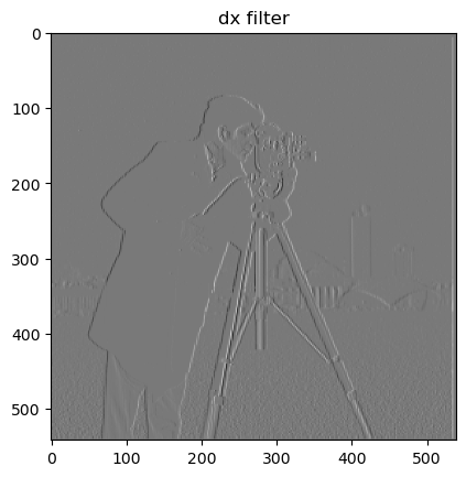
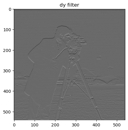
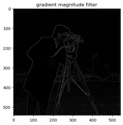
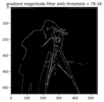
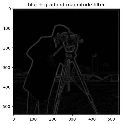
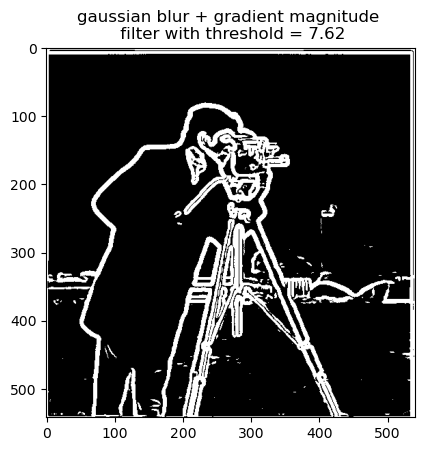
Because images are a discrete sample of continuous objects, we can approximate their gradients using kernels. One of these kernels is the finite difference operator which can be convolved with an image to produce partial derivative approximations. First, we use the filters $D_x = \begin{bmatrix} 1-1\end{bmatrix}$ and $D_y = \begin{bmatrix} 1\\-1\end{bmatrix}$ , to find the partial derivatives with respect to x and y. Next, we find the magnitude of the gradient at each pixel by taking the L-2 Norm of the partials, this results in a cleber approximation of all edges in the screen. Furthermore, setting a threshold makes this result much more clear to the eye. We can use the formula below where p is a pixel.

Part 1.1 Finite Difference Operator

Part 1.2 Derivative of a Gaussian Filter

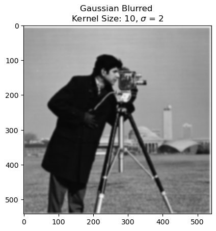
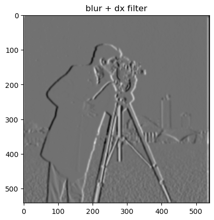
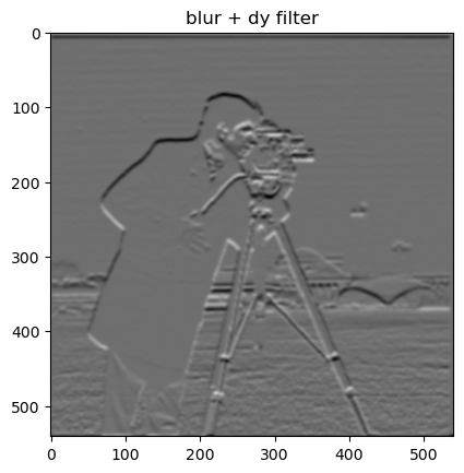
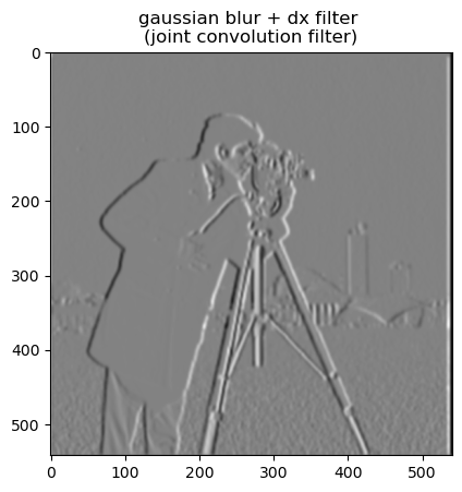
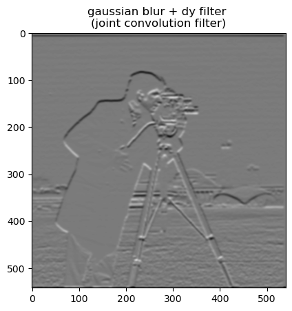
All of the images below use the Gaussian Kernel of Size 10x10 and sigma = 2.0.

We demonstrate that the associativity of convolutions by showing that the joint filters are the same as performing the two operations of blurring and gradient filtering!

Answer to questions:

1. The main difference is the reduction of noise in the edges. More specifically, the edges are emphasized as a result of the blurring, this also means that the edges are less sharp and exact. One can even say that this rounds out the edges and generates a rounded border around the subjects of the image.

Part 2: Fun with Frequencies

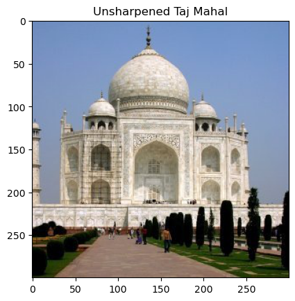
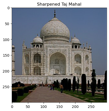
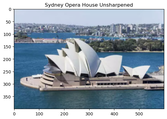
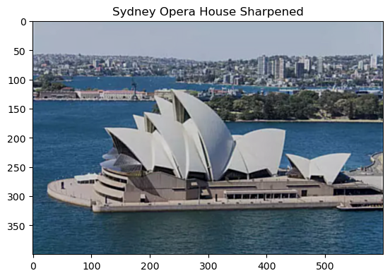
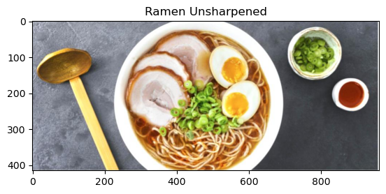
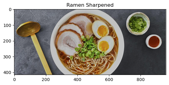
We can increase the sharpness of images by extracting the high frequency components and adding a proportion back to the image because edges are represented by high frequency features. We can compute this by subtracting the gaussian filter result from a unit impulse over a kernel!

Part 2.1: Image Filtering

Part 2.2 Hybrid Images

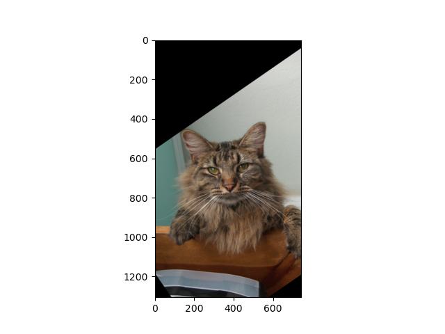
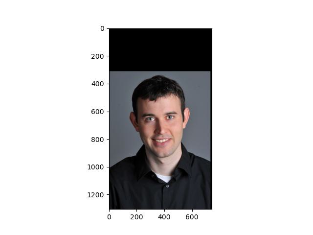
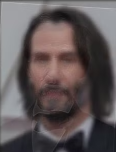
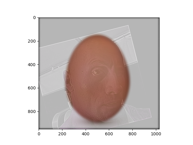
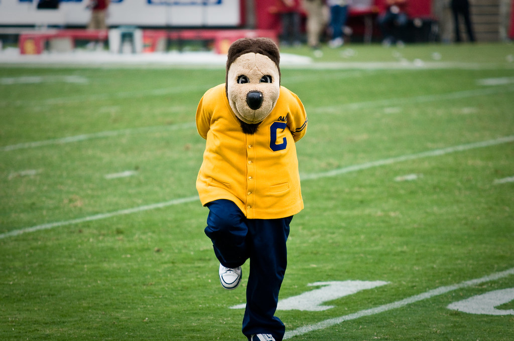
Next, we extract the high frequency components of one image and the low frequency components of another to create hybrid images. The human eye struggles to see high frequency features from far distances, so the low-passed image will be most prominently visible!

Step 1: Align

Map 2 points from each image to line them up!

Step 2: Filter

High Pass Filter Using Impulse - Gaussian Kernel

Low Pass Filter Using Gaussian Kernel

Step 3: Add each layer and fix brightness

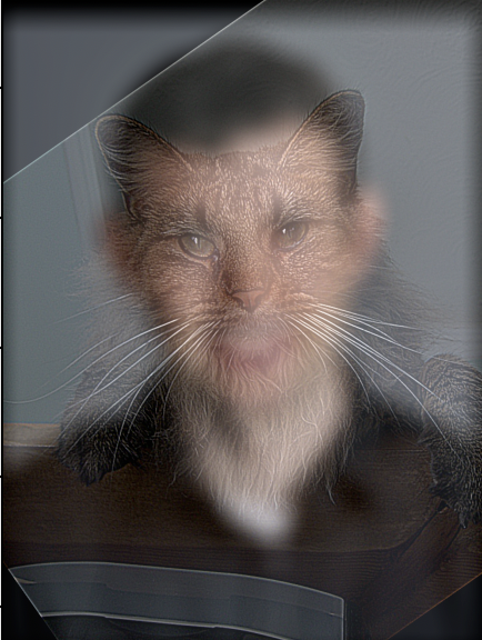
A few samples

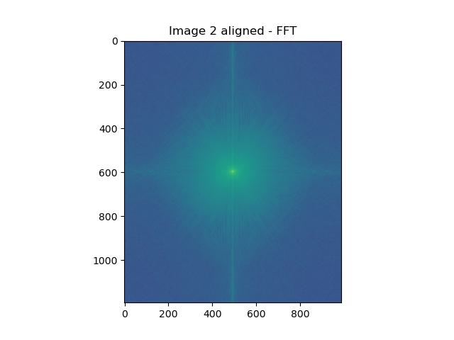
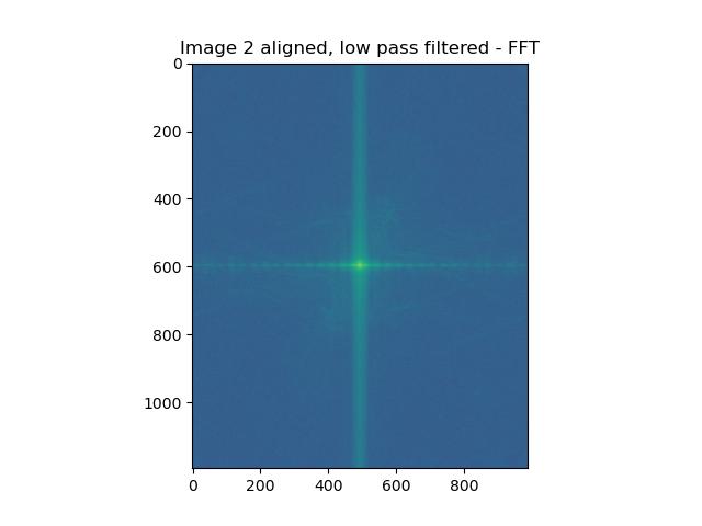
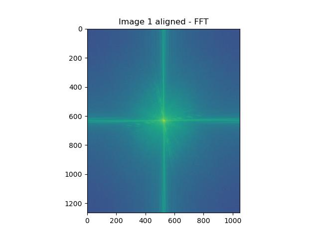
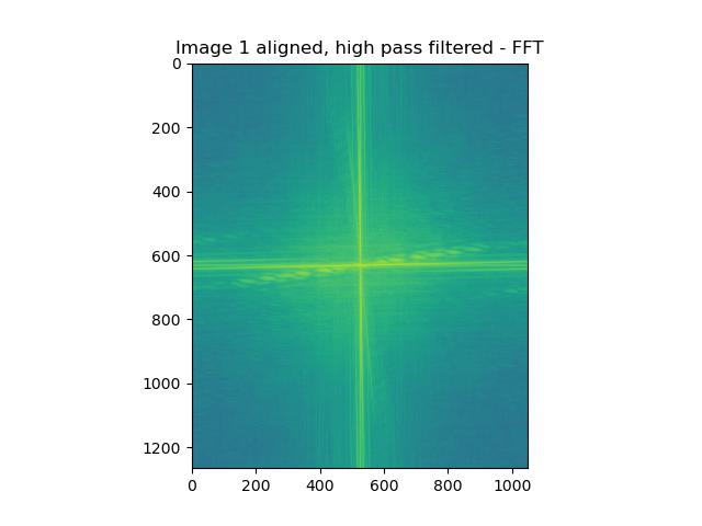
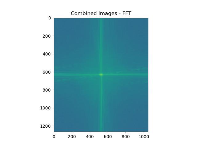
Visualizing Hybrid Images in FFT Space

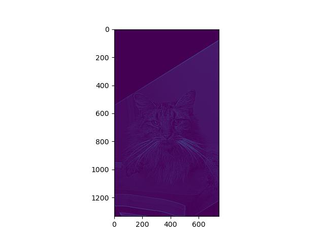
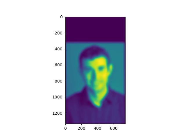
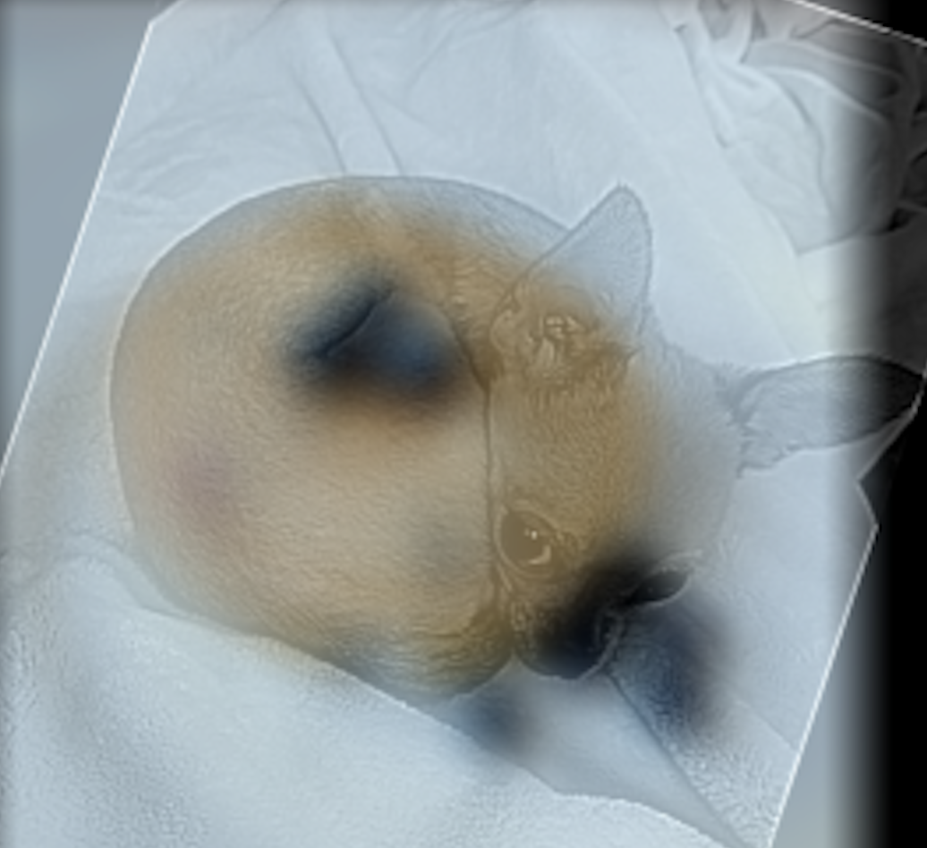
We can also visually see the effects of filtering and combining through the Fourier domain! Below we perform the same operations as above, but we step through the Fourier transforms!

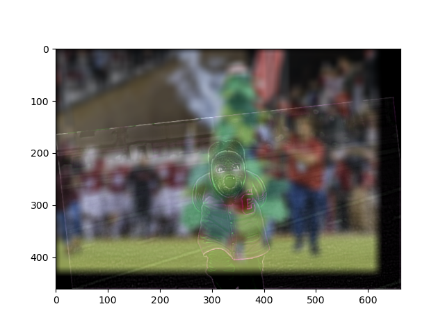
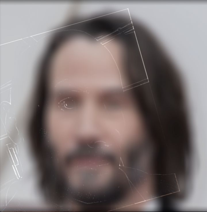
Of course, there were some failures… :(

Part 2.3: Gaussian and Laplacian Stacks

Gaussian and Laplacian Stacks of Apple

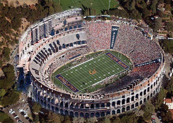
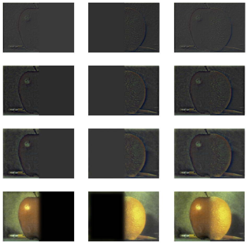
Part 2.4 : Multiresolution Blending and the Orapple Journey

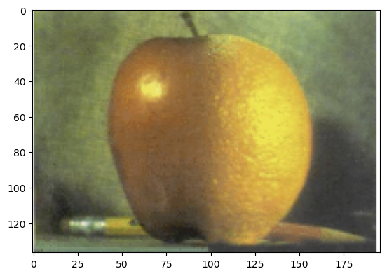
Behold, the Orapple:
Laplacian Stack With Mask applied in element-wise sums per matrix

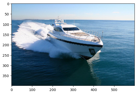
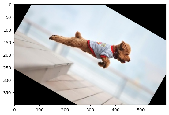
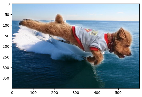
Some more samples!

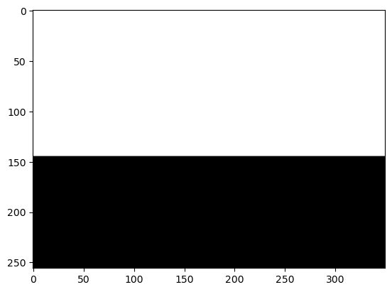
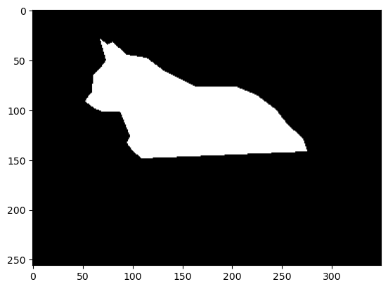
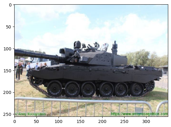
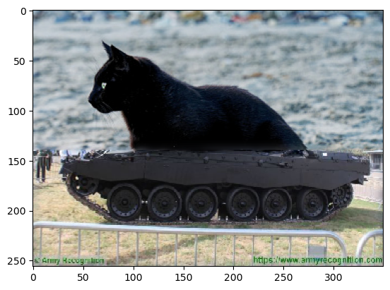
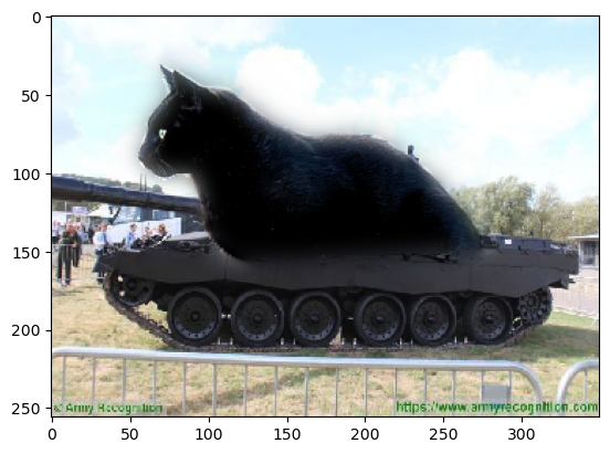
Here we show an example where we can use a simple horizontal mask or a more complex polygon mask on the cat tank. By creating a better mask, the image looks more realistic.

Image 1

Image 2

Project 2