Project 5: Diffusion Models

In this project we explore U-Nets and diffusion models in order to denoise, enhance, and generate images.

Skip to PART B

Project 5A

In this project we explore pretrained denoising models and use them to diffuse entirely new images using a few clever techniques.

Part 0: Setup

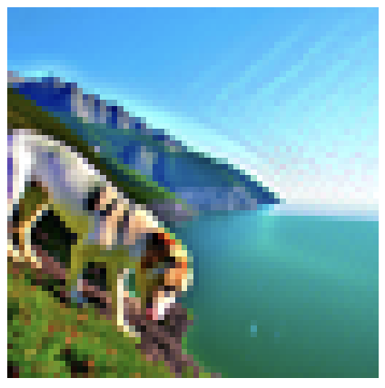
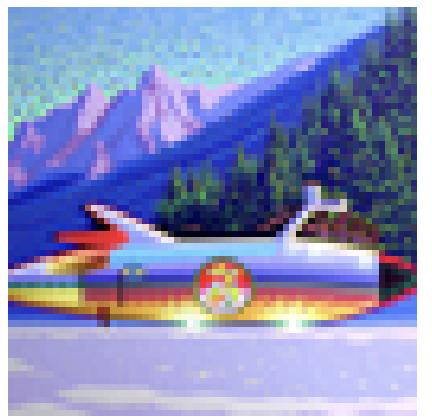
These images seem to capture the task or prompt well. However, there are a few artifacts. Some of these include eyes and facial features not matching up. Because humans have very small features and patterns, it is hard for a model to create a realistic human. However, other objects such as a rocket ship and mountain village look great and show how the model does well with smooth objects with lower-frequency features.

An oil painting of a snowy mountain village

A man wearing a hat

A rocket ship

For this project, I will be using a Seed of 180 in PyTorch.

Part 1: Sampling Loops

Part 1.1 Implementing the Forward Process

The forward process is defined by: $q(x_t | x_0) = N(x_t ; \sqrt{\bar\alpha_t} x_0, (1 - \bar\alpha_t)\mathbf{I})$ . When computing our new images, we can compute the image with:

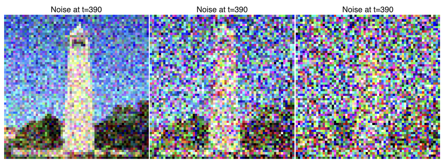
x_t = \sqrt{\bar\alpha_t} x_0 + \sqrt{1 - \bar\alpha_t} \epsilon \quad \text{where}~ \epsilon \sim N(0, 1)

Part 1.2 Classical Denoising

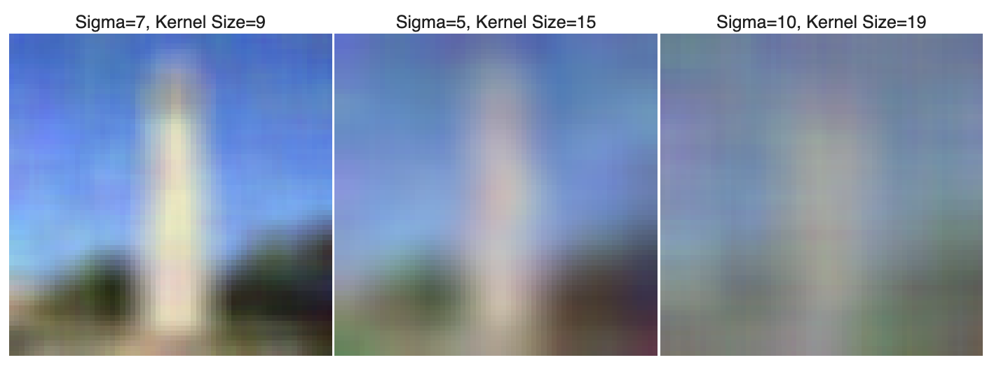
Part 1.3 One-Step Denoising

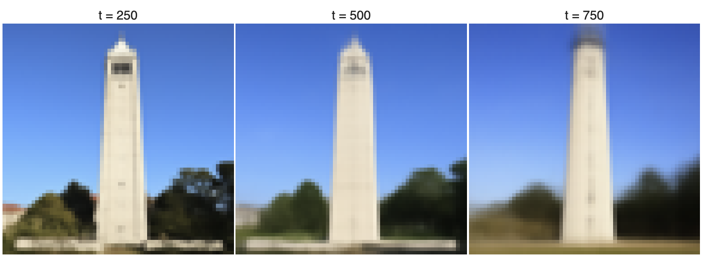
1.4 Iterative Denoising

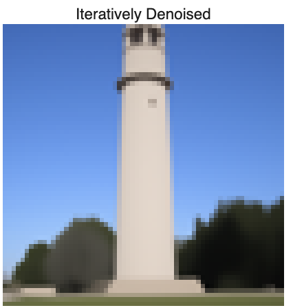
We denoise in iterative and skipped steps. Each step at a time t is defined by:

x_{t'} = \frac{\sqrt{\bar\alpha_{t'}}\beta_t}{1 - \bar\alpha_t} x_0 + \frac{\sqrt{\alpha_t}(1 - \bar\alpha_{t'})}{1 - \bar\alpha_t} x_t + v_\sigma

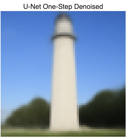
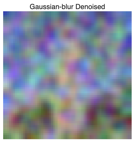
This performs much better than gaussian-blurred and one-step denoising. We will modify this idea to create the rest of the image-generation techniques in this project.

1.5 Diffusion Model Sampling

Random samples starting from pure noise tensors of image size

1.6 Classifier-Free Guidance (CFG)

This modification to the iterative denoising algorithm, we can create much more realistic images than before.

\epsilon = \epsilon_u + \gamma (\epsilon_c - \epsilon_u)

Good when $\gamma > 1$

1.7 Image-to-Image Translation

1.7.1 Editing Hand-Drawn and Web Images

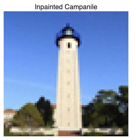
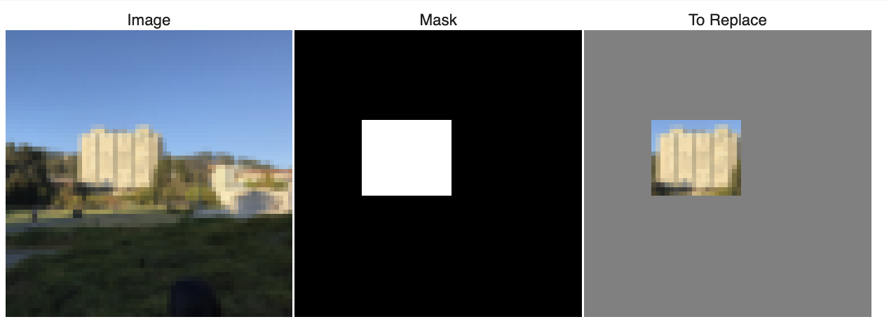
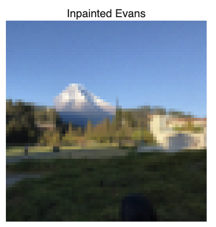
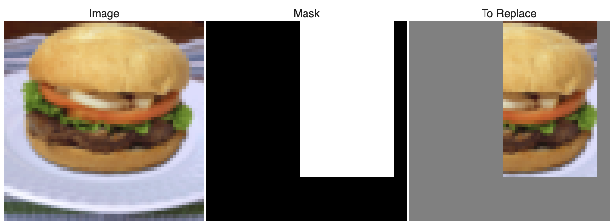
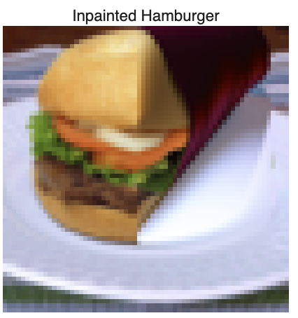
1.7.2 Inpainting

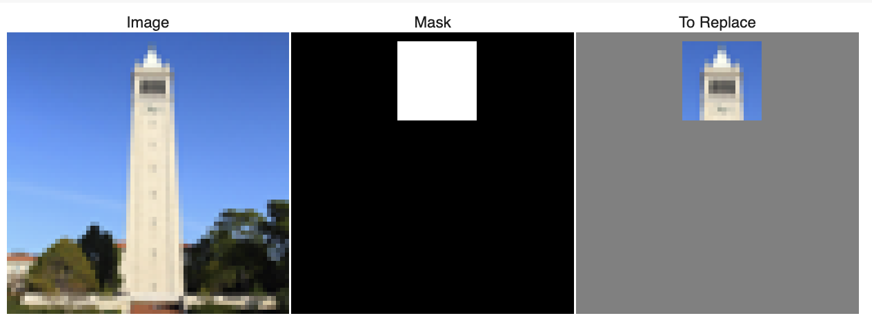
x_t \leftarrow \textbf{m} x_t + (1 - \textbf{m}) \text{forward}(x_{orig}, t) \tag{5}

By using masks, we can remove parts of the old image, and force the reconstruction to keep a slightly less noisy version of the original image each time. Like this, we can force the model to fill in the gaps based on how the rest of the noise changes!

Campanile turned into lighthouse

Replacing Evans with Mt. Fuji!

Burger turned into a kofta kabob wrap

1.7.3 Text-Conditional Image-to-image Translation

“Draw a rocket ship”

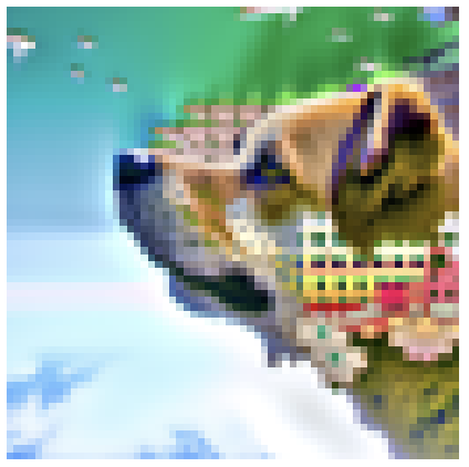
“A photo of a dog”

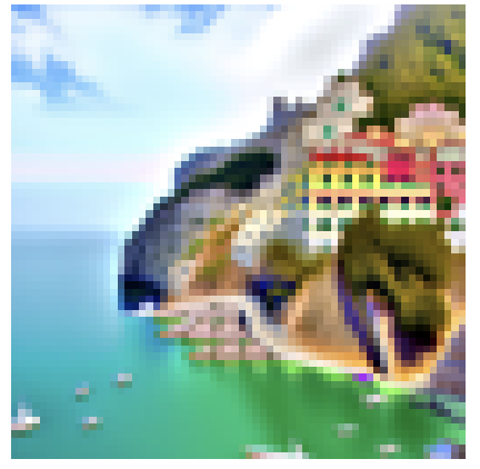
“Amalfi Coast”

Original Image: A picture of the book “The Elements of Statistical Learning” by Hastie, Tibshirani, and Friedman

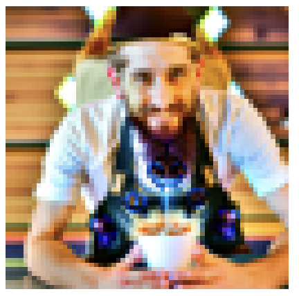
Using prompt: “A photo of a hipster barista”

“A Pencil”

1.8 Visual Anagrams

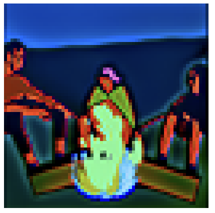
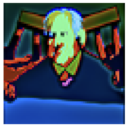
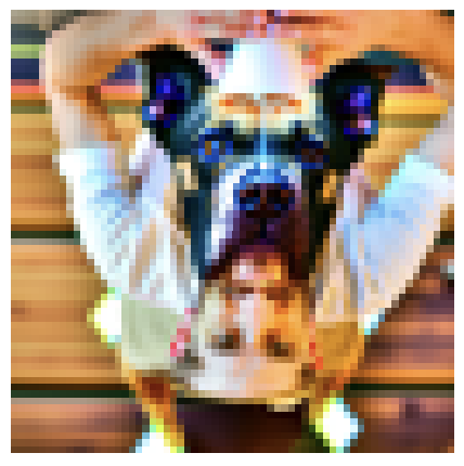
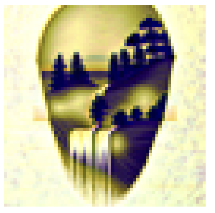
By formulating two optimization problems as one with a singular epsilon, we can find the “compromise” solution between two objectives. This allows us to generate images which appear to be one thing when viewed normally, and another from afar!

We use the following formulas:

\epsilon_1 = \text{UNet}(x_t, t, p_1) \\ \epsilon_2 = \text{flip}(\text{UNet}(\text{flip}(x_t), t, p_2)) \\ \epsilon = \frac{(\epsilon_1 + \epsilon_2)}{2}

An Oil Painting of People Sitting Around a Fire

An Oil Painting of an Old Man

A Photo of a Dog

A Photo of a Hipster Barista

Amalfi Coast

A Photo of a Dog

1.9 Hybrid Images

Going back to the second project, we learned how to create low and high-pass filters for imaging. Applying these principles, we can create images with high and low-frequency features based on two different prompts.

We use:

\epsilon_1 = \text{UNet}(x_t, t, p_1) \\ \epsilon_2 = \text{UNet}(x_t, t, p_2) \\ \epsilon = f_\text{lowpass}(\epsilon_1) + f_\text{highpass}(\epsilon_2)

Low Pass: “A lithograph of a skull”

High Pass: “A lithograph of waterfalls”

Low pass: “A photo of the alfari cost”

High Pass: “A photo of a dog”

Low Pass: “An oil painting of a snowy mountain village”

High Pass: “A rocket ship”

Project 5B: Diffusion Models from Scratch

1.2 building a Unet from scratch

Visualize example

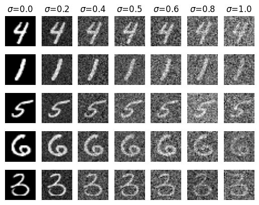
1.2.1 Train the U-Net

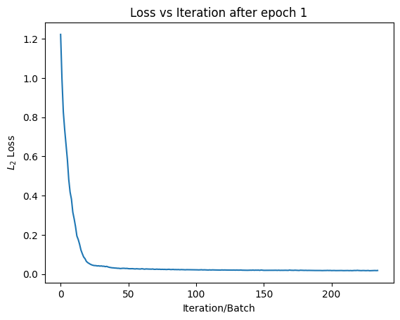
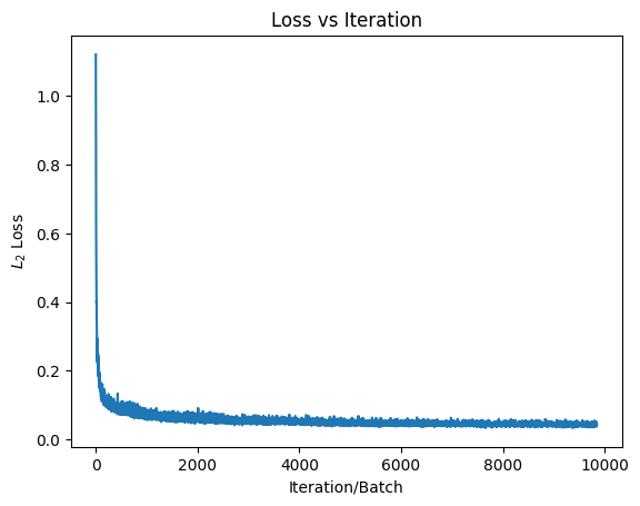
Training Algorithm 1:

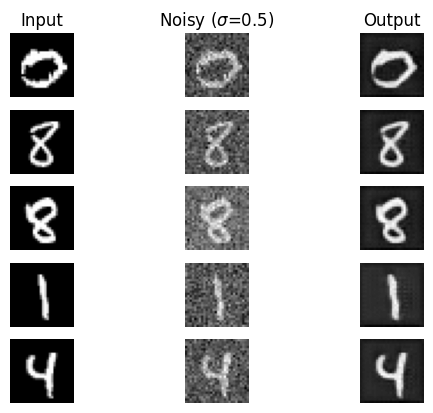
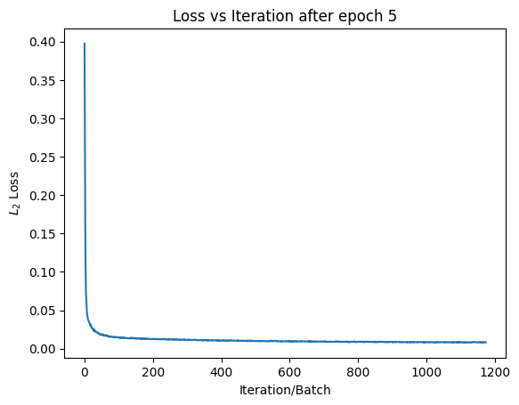
Results after 1 Epoch

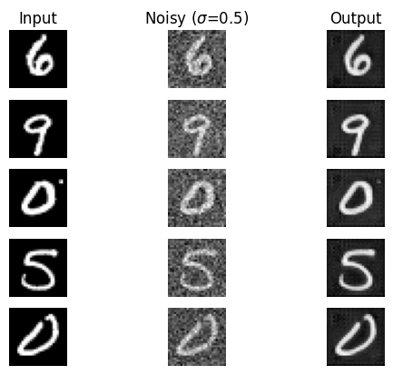
Results after 5 Epochs

1.2.2 Out-of-Distribution Testing

By testing with values of noise other than $\sigma=0.5$ , we can analyze how well the model generalizes to all degrees of noise. By training at $\sigma = 0.5$ , we can easily denoise levels of noise under than level without adding any discernable artifacts. However, once the noise gets quite substantial, the images begin to develop artifacts and inaccuracies. However, the images appear to represent the same digit as before.

Part 2: Training a Diffusion Model

In this part, we implement diffusion models which will use time-conditioning in order to suplement the iterative process which we used earlier.

2.1 Adding Time Conditioning to UNet

In the previous part, we created a model which could denoise. However, we can use this process to find the noise itself and integrate this with the following formula to implement iterative denoising!

Time-Conditioned Model Graph

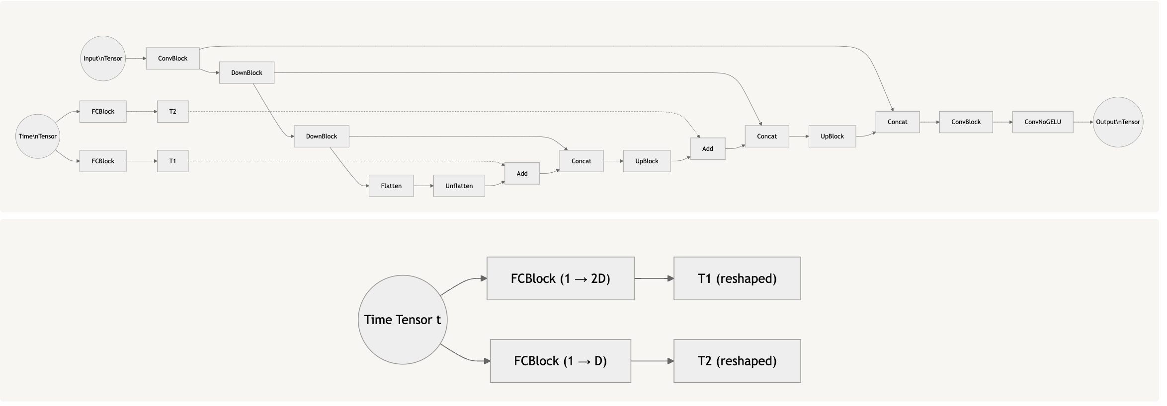
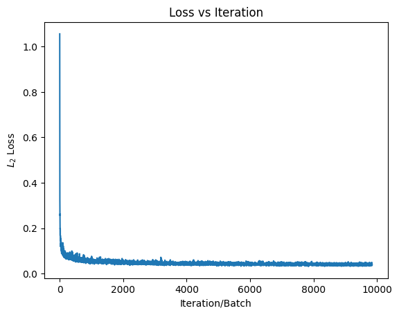
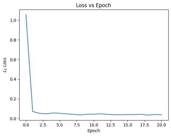
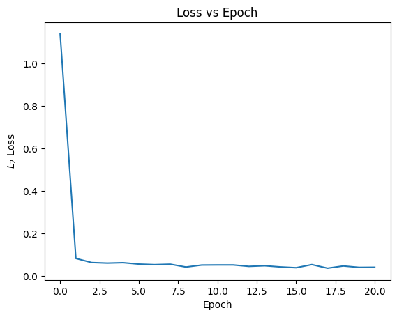
2.2 Training the Time Conditioned UNet

2.3 Sampling from the Time Conditioned UNet

\textbf{Algorithm 1: Time-Conditioned Training} \\ \begin{align*} &\text{Precompute }\bar{\alpha}\\ x_0 &= \text{clean image from training set} \\t &= \mathrm{Uniform}(\{1, \ldots, T\}) \\\epsilon &= \mathcal{N}(0, I) \\x_t &= \sqrt{\bar{\alpha}_t} x_0 + \sqrt{1 - \bar{\alpha}_t} \epsilon \\\hat{\epsilon} &= \mathrm{UNet}_{\theta}(x_t, t)\end{align*} \\ \textbf{Gradient Step with Adam on:} \\\nabla_{\theta} \|\epsilon - \hat{\epsilon} \|

\textbf{Algorithm 2: Time-Conditioned Sampling} \\ \begin{align*}& \text{Precompute } \beta, \alpha, \text{ and } \bar{\alpha} \\& x_T \sim \mathcal{N}(0, I) \\& \text{for } t \text{ from } T \text{ to } 1, \text{ step size } -1 \text{ do} \\& \ \ \ z \sim \mathcal{N}(0, I) \ \text{if } t > 1, \ \text{else } z = 0 \\& \ \ \ \hat{x}_0 = \frac{1}{\sqrt{\alpha_t}} \left( x_t - \sqrt{1 - \bar{\alpha}_t} \, \mathrm{UNet}_\theta(x_t, t) \right) \\& \ \ \ x_{t-1} = \frac{\sqrt{\bar{\alpha}_{t-1}}\beta_t}{\sqrt{1 - \bar{\alpha}_t}} \hat{x}_0 + \sqrt{\alpha_t \left( 1 - \bar{\alpha}_{t-1} \right)} x_t + \sqrt{\beta_t} z \\& \text{end for} \\& \text{return } x_0\end{align*}

Why compute noise on the fly instead of preprocessing in batches for better GPU Utilization?

By computing the noise on the fly, we introduce dynamic variability to the training data, allowing our model to generalize better and reducing overall bias. While this approach is computationally more intensive, it enables the algorithm to discover a broader range of relationships in the data.
For instance, with 50,000 samples and precomputed noise, we're limited to exactly those 50,000 variations. However, by generating random noise during training, we effectively create unlimited unique samples drawn from the noise distribution. This helps the model encounter a broader range of scenarios and learn more
generalizable patterns than it would with a fixed set of precomputed noise samples.

This approach is conceptually similar to bootstrapping from the manifold of random noise matrices based on Gaussian distributions - we're repeatedly sampling from the underlying distribution to better approximate the true noise manifold. Just as bootstrapping helps us estimate population parameters by resampling from observed data, generating noise on the fly helps us better explore the full domain of possible noise patterns, leading to more robust learning. (CS 189!)

Moreover, precomputing and storing noise for each timestep would be memory-intensive - with 300 timesteps and 50,000 samples, we'd need to store 15 million noise tensors (300 × 50,000). For small 28×28 images, this might be manageable, but when working with high-resolution data or larger batch sizes, the memory requirements can become prohibitive. Not only would this significantly increase memory needs, but using fixed noise patterns for each timestep could potentially lead to overfitting, as the model might learn to exploit specific patterns in the precomputed noise rather than developing robustness to genuine random variations.

However, we can get around the inefficiencies of on-the-fly modifications by computing the necessary data in parallel with torch batch operations, allowing the hardware to make better use of multithreading or other methods of parallelism. (CS 152!)

Results at Epoch 5

Results at Epoch 20

2.4 Adding Class-Conditioning to UNet

Class and Time-based Conditioned Graph

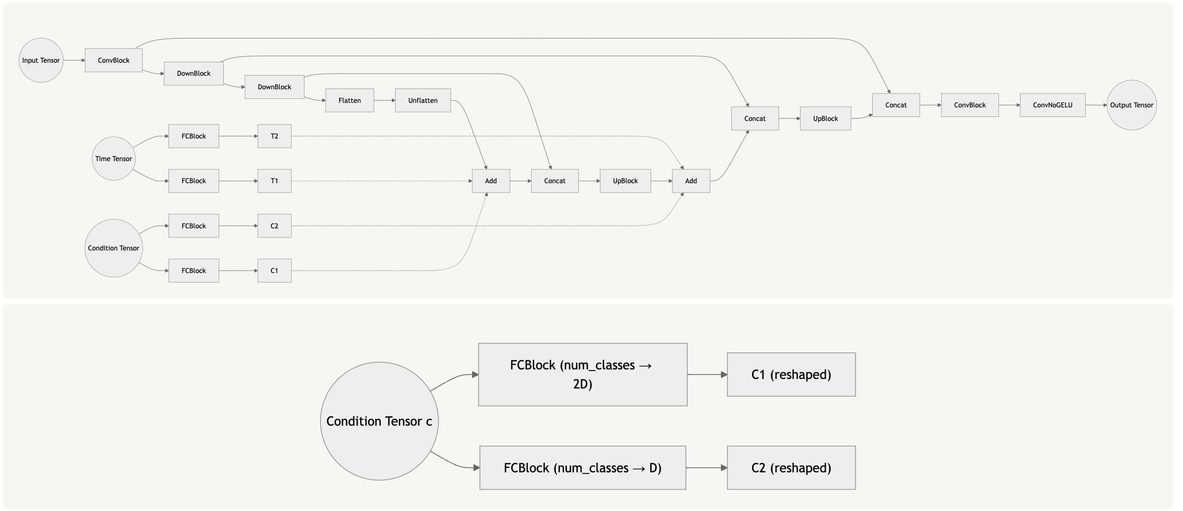
In order to condition on class, we added a new block which allows us to capture information about each new class. However, because this information does not match the size of the layer we want to condition, we must transform it using the block described above.

2.5 Sampling from the Class Conditioned UNet

\textbf{Algorithm 3: Class-Conditioned Training} \\ \begin{align*} &\text{Precompute }\bar{\alpha}\\ x_0 &= \text{clean image from training set} \\ c &= \text{one-hot vector for class if provided with class label} \\ &\text{Make c = 0 with probability } P =0.1 \\ t &= \mathrm{Uniform}(\{1, \ldots, T\}) \\\epsilon &= \mathcal{N}(0, I) \\x_t &= \sqrt{\bar{\alpha}_t} x_0 + \sqrt{1 - \bar{\alpha}_t} \epsilon \\\hat{\epsilon} &= \mathrm{UNet}_{\theta}(x_t, t)\end{align*} \\ \textbf{Gradient Step with Adam on:} \\\nabla_{\theta} \|\epsilon - \hat{\epsilon} \|

\textbf{Algorithm 4: Class-Conditioned Sampling} \\\begin{align*}& \text{input: one-hot vector } c, \text{ classifier-free guidance scale } \gamma \\& x_T \sim \mathcal{N}(0, I) \\& \text{for } t \text{ from } T \text{ to } 1, \text{ step size } -1 \text{ do} \\& \ \ \ z \sim \mathcal{N}(0, I) \ \text{if } t > 1, \ \text{else } z = 0 \\& \ \ \ \epsilon_u = \mathrm{UNet}_\theta(x_t, t, 0) \\& \ \ \ \epsilon_c = \ \mathrm{UNet}_\theta(x_t, t, c) \\& \ \ \ \epsilon = \epsilon_u + \gamma \left( \epsilon_c - \epsilon_u \right) \\& \ \ \ \hat{x}_0 = \frac{1}{\sqrt{\alpha_t}} \left( x_t - \sqrt{1 - \bar{\alpha}_t} \epsilon \right) \\& \ \ \ x_{t-1} = \frac{\sqrt{\bar{\alpha}_{t-1}}\beta_t}{\sqrt{1 - \bar{\alpha}_t}} \hat{x}_0 + \sqrt{\alpha_t \left( 1 - \bar{\alpha}_{t-1} \right)} x_t + \sqrt{\beta_t} z \\& \text{end for} \\& \text{return } x_0\end{align*}

Again, we compute noise and transformations on the fly in order to prevent overfitting!

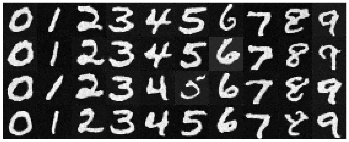
Sampling at Epoch 5

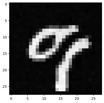
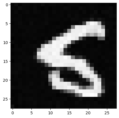
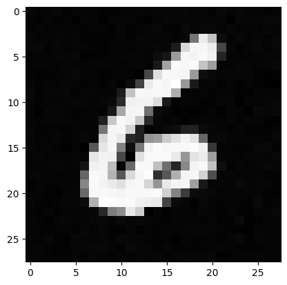
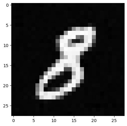
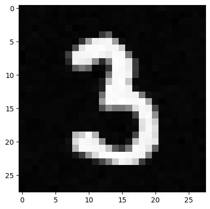
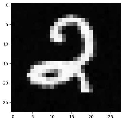
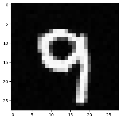
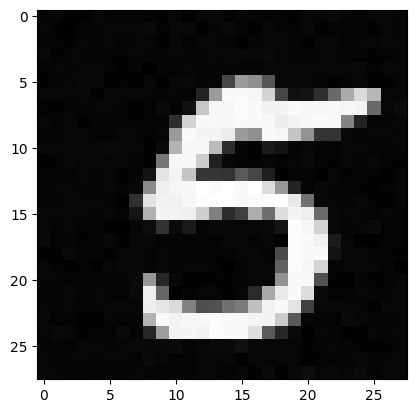
The images at Epoch 5 appear to be recognizable, but some crucial parts of the numbers are perturbed. By training on more data and noise, this can be accounted for.

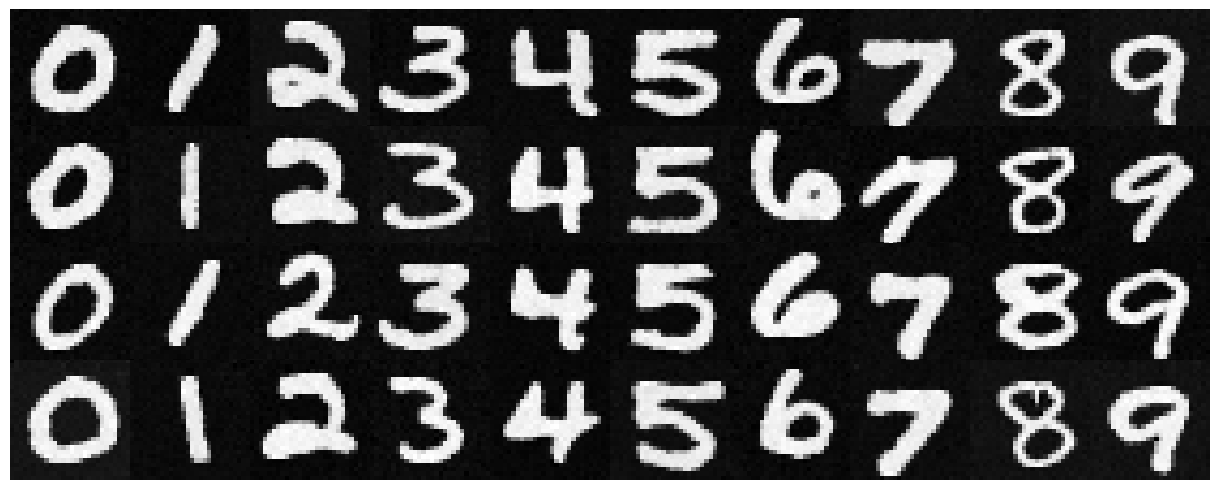
Sampling at Epoch 20

At Epoch 20, we see that a lot of the previous artifacts are removed. A lot of the angles are sharper, but the use of the $\gamma=5$ based reconstruction leads to numbers which look a bit different from those from the standard time-conditioned samples.

Bells and Whistles: GIF

Thoughts and Conclusion:

Overall, this was a rewarding project which helped me learn a lot more about diffusion models and UNets than I did before. Looking forward to working with this technology again in the future!