David Martinez, Fall 2024

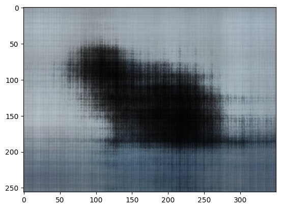
Part 1: 2D Nerf

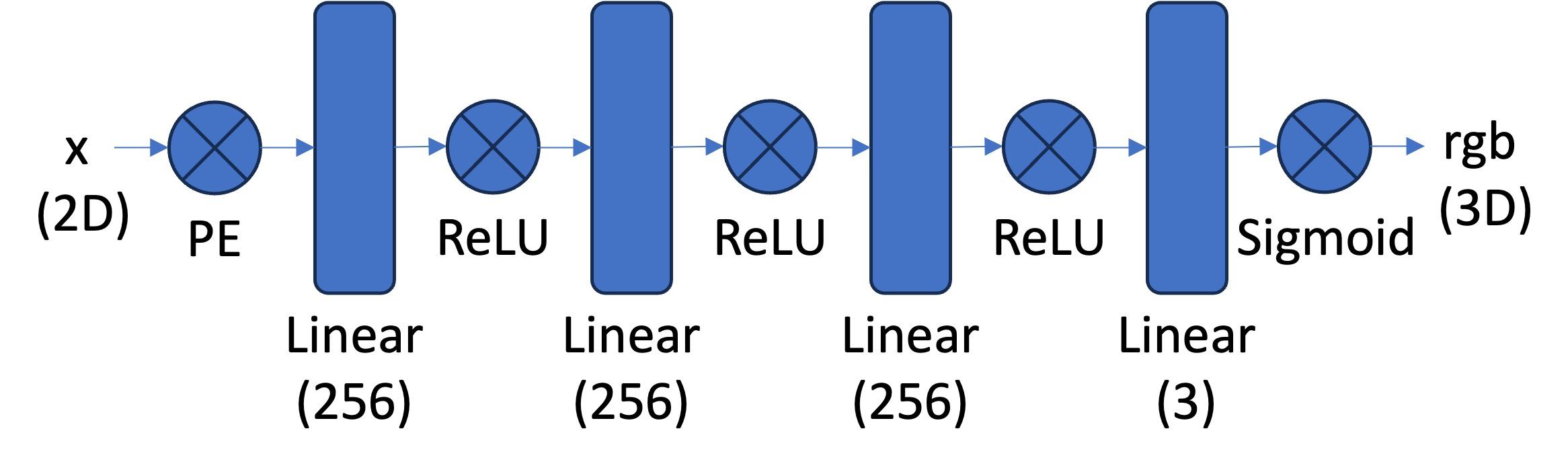
Since Neural Networks tend to learn low-frequency features better, we can help our network learn fine details by using a positional encoding as such:

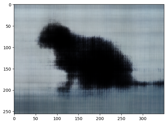
Before creating the 3D NeRF, I created a 2D nerf where we can reproduce an image with just a network and some embeddings. I chose to follow the above architecturre which uses ReLU to ensure that we have real value pixels in the image. Finally, the sigmoid activation ensures that the range of our output is in the range of 0 to 1. (This makes sense for our normalize pixels!)

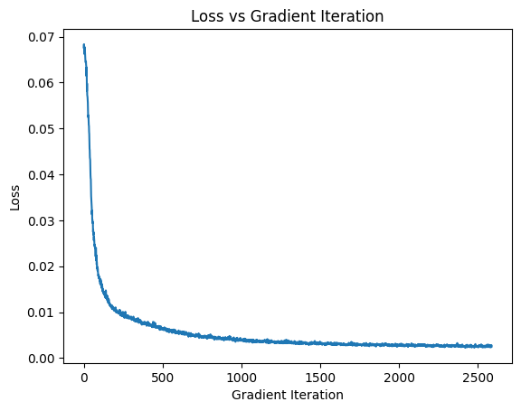
I chose to have the following hyperparamters:

lr_1 = 0.001
optimizer = torch.optim.Adam(model_0.parameters(), lr=lr_1)

This learning rate worked for all of the images I tried. While Gradient descent works fine, I chose to use Adam because it performs well on these tasks and lets us use momentum to our advantage!

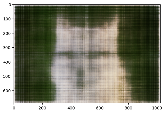
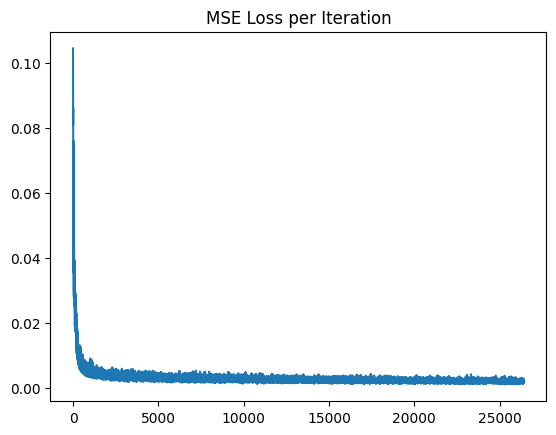
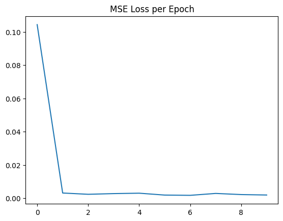
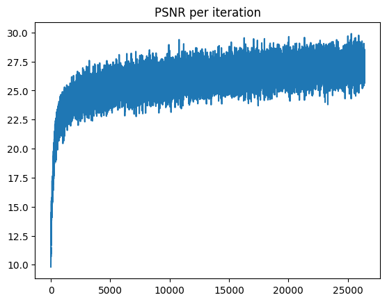
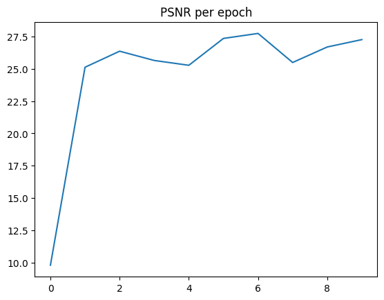
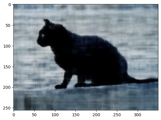
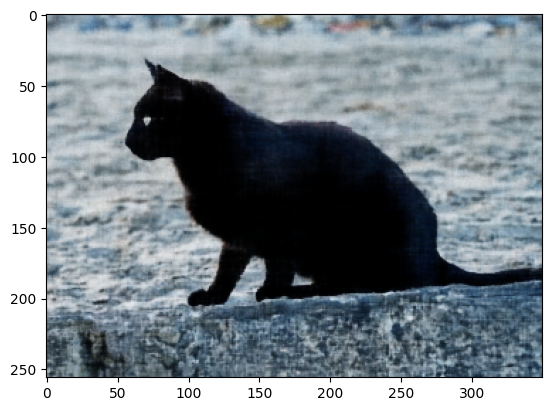
Image 2: Cat

Part 2: Fit a Neural Radiance Field from Multi-view Images

Part 2.1: Create Rays from Cameras

Camera to World Coordinates

We can express the relationship between coordinates in the real world and a camera’s view with the extrinsic world-to-camera matrix. We make use of the inverse in order to map the reverse process!

Here, $\R_{3\times3}$ defines the rotations and t defines the translation of the camera in the 3D space.

Pixel to Camera Coordinates

We can model a simple pinhole camera with the following camera matrix:

We can combine this matrix with real world vectors to recover the pixel coordinate in the image space.

Pixel to Ray Coordinates Pipeline

Next, we combine these two processes to recover the simulated rays which generated any pixel at index [i][j] of our images. Because rays coming from a pinhole have a shared center of projection, we can recover the shared ray origin:

Then, we use our camera to world pipeline to get our ray directions:

Part 2.2: Sampling

Sampling Rays from Images

Since we will want to process many images, it would be hard to fit all of the possible rays from our images onto a GPU. As so, we must use Batched Gradient decent, or a variant of it through batches with the Adam Optimizer. In order to ensure properly learning and correct view coverage, we randomly sample from our images to create batches that have N//M rays per image where N is the total number of rays and M is the number of images. For this, I chose to randomly sample from each image, collecting the ray origins and ray directions, along with the corresponding pixel from the image. These rays are collected into batches for the next step, where we collect points.

Sampling Points along Rays

The second stage of the sampling process is finding points along which we could sample our network. Since we want our network to learn 3D geometry/volume, we must query points all along the ray. For this project, 32 or 64 samples per ray worked pretty well. However, since we want our model to work well for novel view synthesis, we add a bit of noise to each sample point so that the network implicitly “splats” the geometry and learns a sample with less variance. In a way, this is like applying regularization, as it forces the model to adapt to points which is has never seen before. Finally, these points are queried to the network, yielding sigmas and RGBs which are going to be used for the clever approximation of volume in the next step Volume Renderer Step. Note that sigma is going to be the opacity and rgb is the color observed. This is quite similar to how PNGs represent transparency— except we are stacking these pixels to create real color in the next steps.

Part 2.3: Putting the Dataloader Together

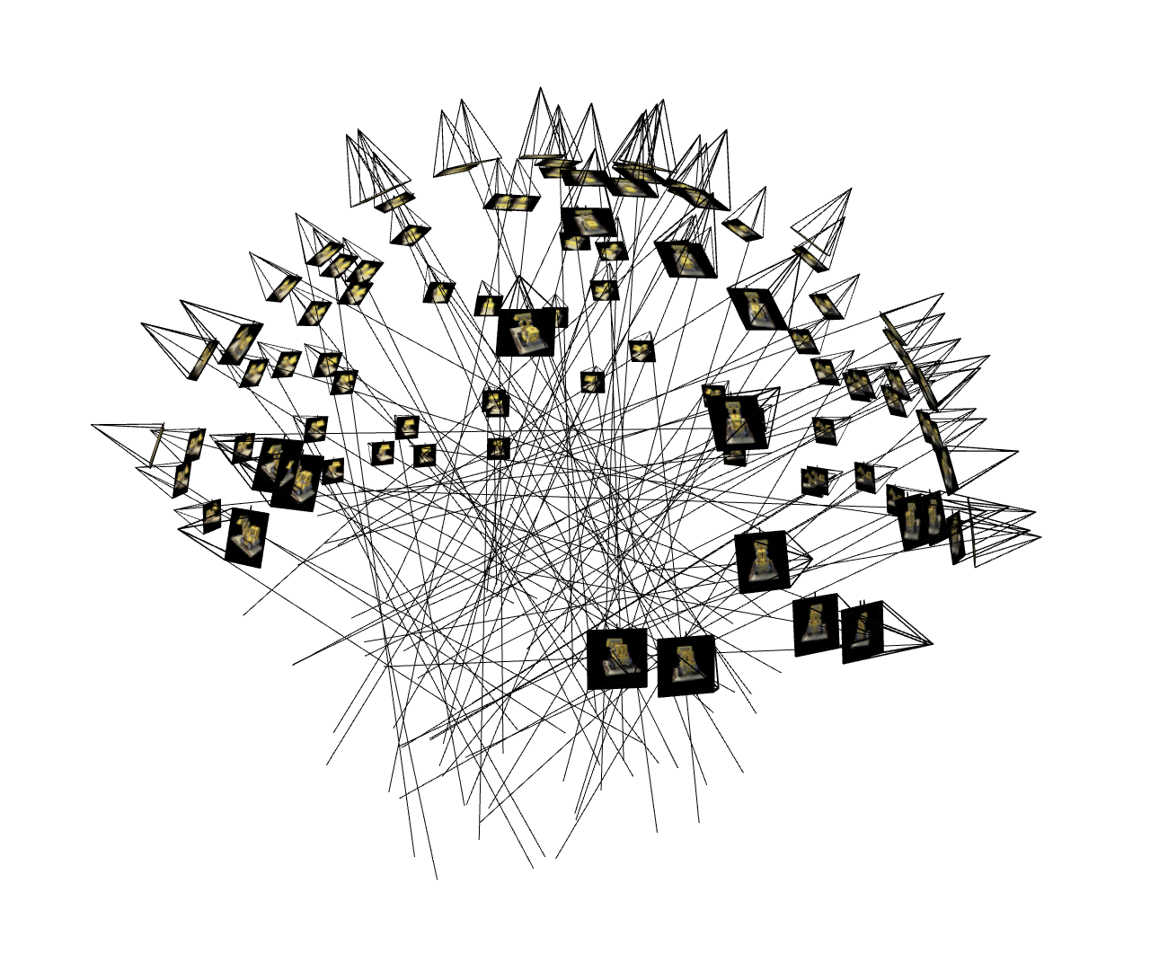
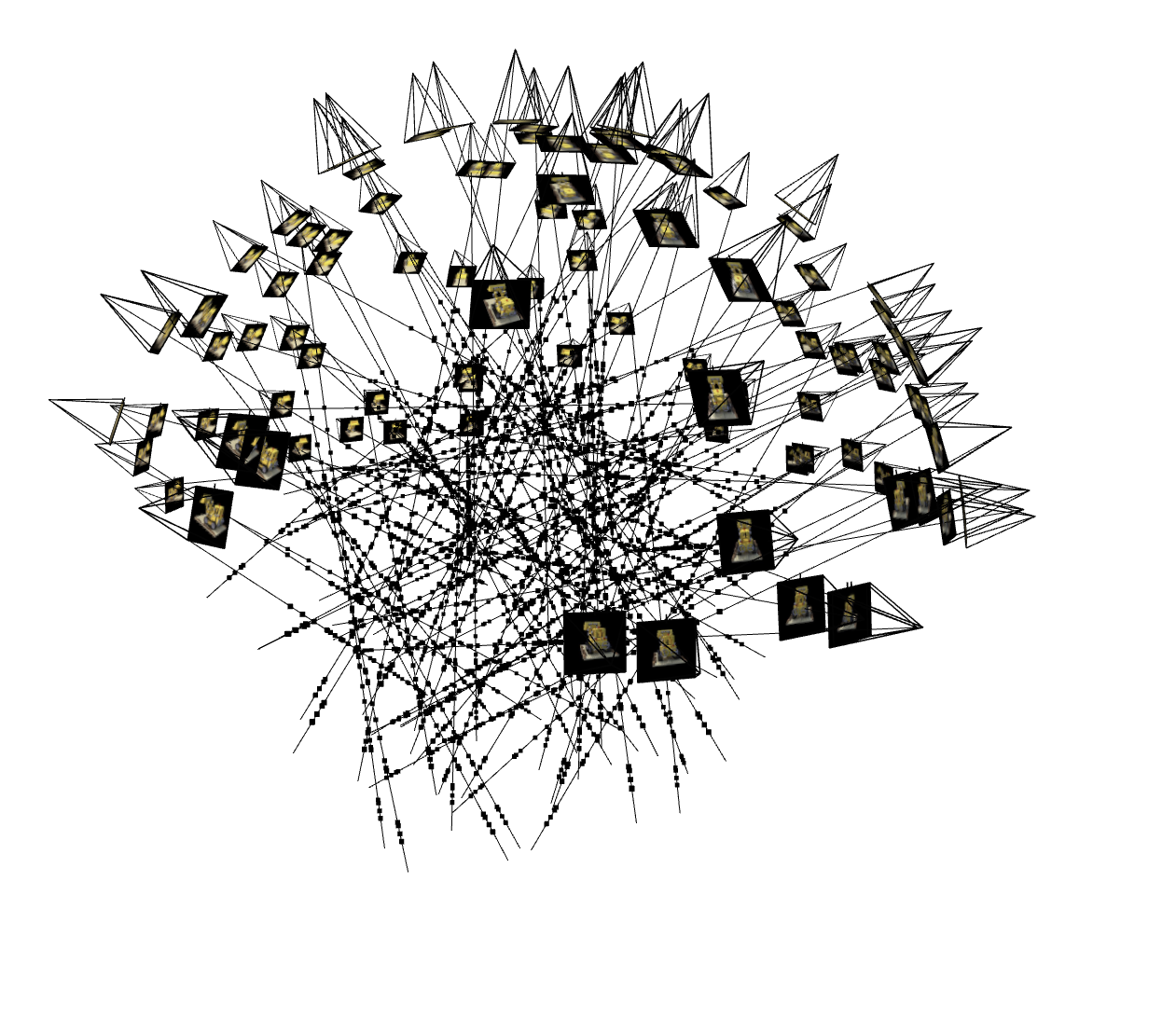
Here we can see the output of our sampling, with rays on the left and the discrete samples on the right. If we add more samples, the space would be full of more dots, likely hard to interpret. However, we can see that the uneven intervals are the result of our noisy sampling!

Part 2.4: Neural Radiance Field

Now, we need some way of capturing how something looks form each angle and position, but this would be a lot of data to hash directly, plus we would be limited to the resolution of our original samples. So, we need a way to capture a continuous and memory-efficient approximation of these densities and colors. For this, we can use Neural networks with positional encodings, which allow the network to combat the bias to learn low-dimensional features.

Why does this work?

Universal Approximation Theorem:

• Networks with a width of n + 4 and ReLU activation functions can approximate any Lebesgue-integrable function on an n-dimensional input space, given an increasing network depth. Additionally, ReLU networks with a width of n + 1 suffice to approximate any continuous function of n-dimensional input variables.

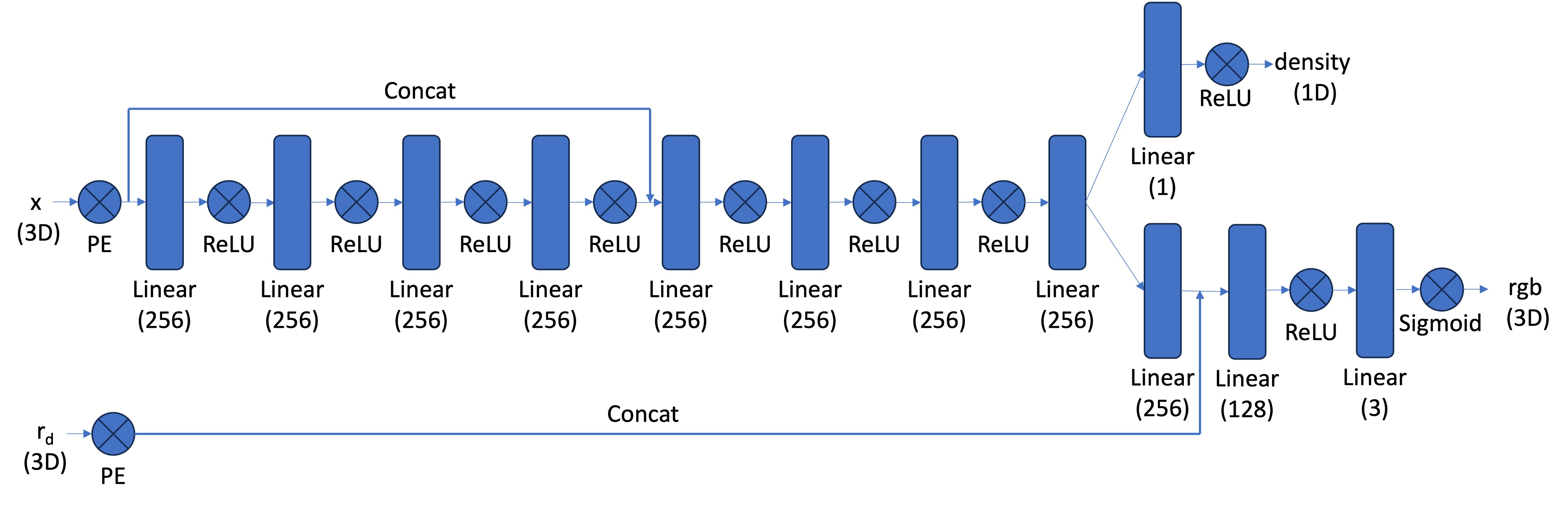
I opted for the following modified architecture which is combines positional encodings on both the 3D coordinate and the ray direction:

class NeRF_3D(nn.Module):
    def __init__(self, encode_size):
        super().__init__()
        self.MLP1 = torch.nn.Sequential(
            nn.Linear(encode_size, 256),
            nn.ReLU(),
            nn.Linear(256, 512),
            nn.ReLU(),
            nn.Linear(512, 512),
            nn.ReLU(),
            nn.Linear(512, 256),
            nn.ReLU(),
            nn.Linear(256, 256),
            nn.ReLU(),
            nn.Linear(256, 256),
            nn.ReLU(),
            nn.Linear(256, 256),
            nn.ReLU(),
            nn.Linear(256, 256),
            nn.ReLU(),
        )
        self.MLP2 = torch.nn.Sequential(
            nn.Linear(encode_size+ 256, 256),
            nn.ReLU(),
            nn.Linear(256, 256),
            nn.ReLU(),
            nn.Linear(256, 256),
            nn.ReLU(),
            nn.Linear(256, 256)
        )
        self.density_net = torch.nn.Sequential(
            nn.Linear(256, 256),
            nn.ReLU(),
            nn.Linear(256, 1),
            nn.ReLU()
        )
        self.pre_rgb_layer = torch.nn.Sequential(
            nn.Linear(256, 256)
        )
        self.rgb_net = torch.nn.Sequential(
            nn.Linear(256 + 27, 256),
            nn.ReLU(),
            nn.Linear(256, 128),
            nn.ReLU(),
            nn.Linear(128, 3),
            nn.Sigmoid()
        )
    def forward(self, x, r_d):
        pe_x = positional_encoding(x, L=10)
        pe_r_d = positional_encoding(r_d, L=4)
        x = pe_x.clone()
        x = self.MLP1(x)
        x = torch.concat((x, pe_x), dim=1) # share batch dim
        x = self.MLP2(x)
        # handle density
        d = self.density_net(x)
        # handle rgb
        r = self.pre_rgb_layer(x)
        r = torch.concat((r, pe_r_d), dim=1)
        rgb = self.rgb_net(r)
        return d, rgb

Part 2.5: Volumetric Rendering

In order to figure out what a pixels will look like from any unique view, we must integrate over the voxels that are “hit” by each ray. This process involves capturing the opacity and color of each pixel, resulting in a final color that looks like the color of the pixel which corresponds to that ray. This integration can be described as volumetric rendering:

However, because we are unable to integrate this function with infinite steps or voxels, we will opt for a discrete approximation with a sampling rate of sampling rate of n = 32 or n = 64.

FUNCTION volrend(sigmas, rgbs, step_size):
    # Step 1: Compute cumulative transmittance along the ray
    sdel = -CUMSUM(sigmas * step_size, axis=1)
    pad_shape = SHAPE(sdel)
    pad_shape[1] = 1  # Adjust shape for padding
    sdel = CONCATENATE(ZEROS(pad_shape), sdel, axis=1)[:, :-1]
    T = EXP(sdel)
    
    # Step 3: Compute coefficients for volume rendering
    coeffs = 1 - EXP(-sigmas * step_size)

    # Step 4: Compute weighted contributions of colors
    res = T * coeffs * rgbs

    # Step 5: Accumulate contributions to get final color
    output_color = SUM(res, axis=1)

    RETURN output_color

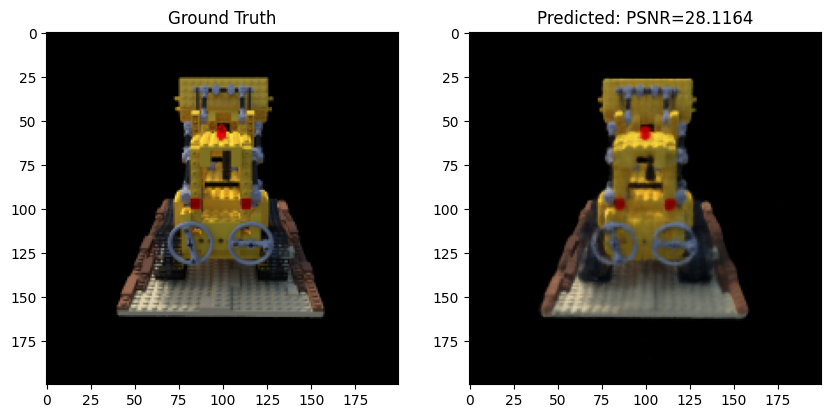
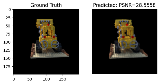
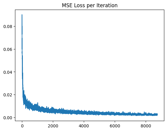
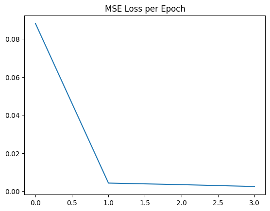
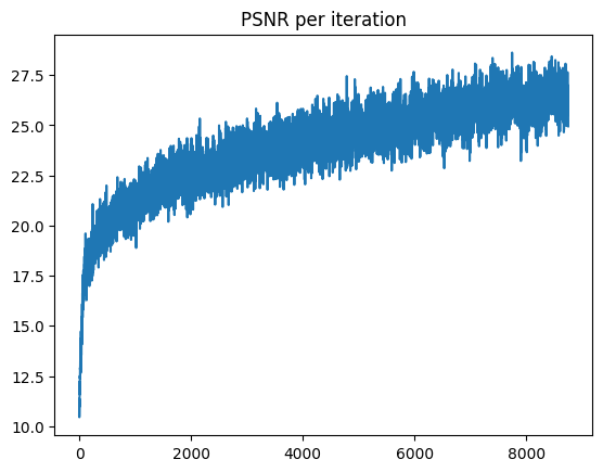
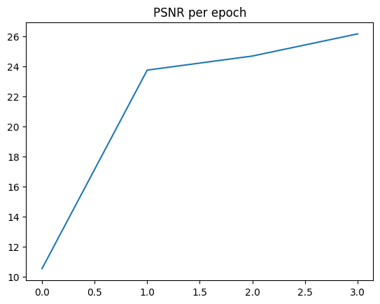
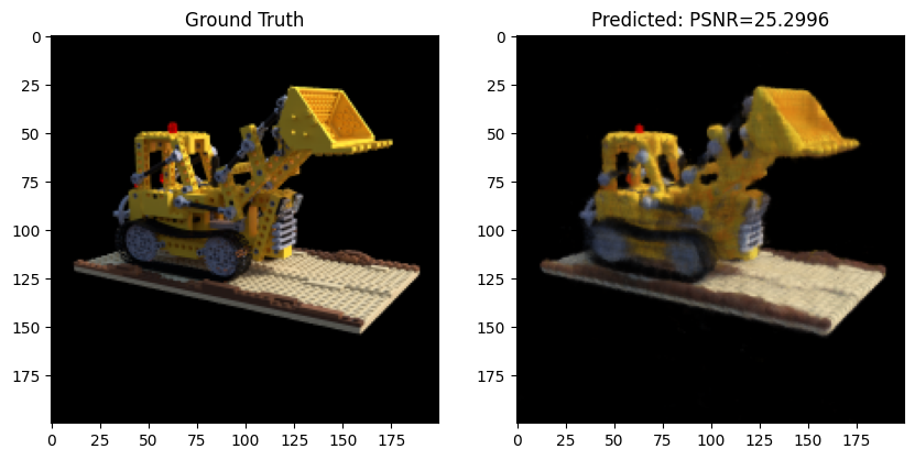
Results:

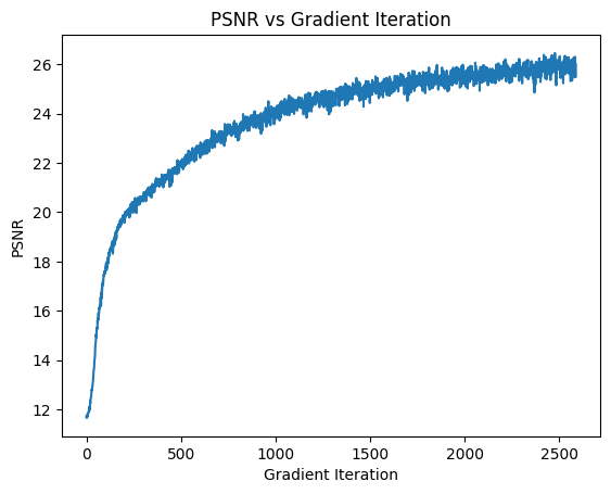
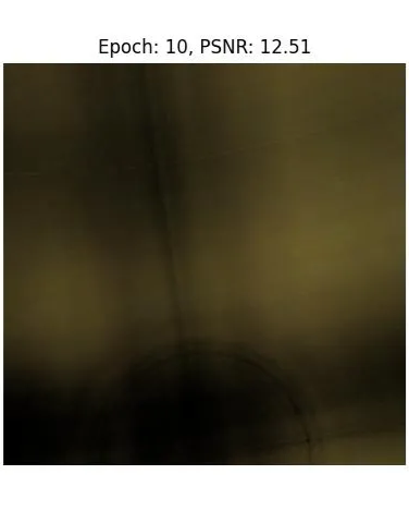
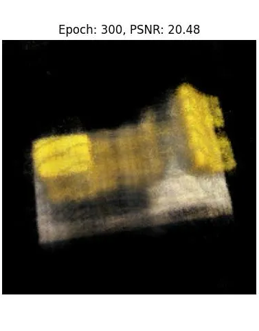
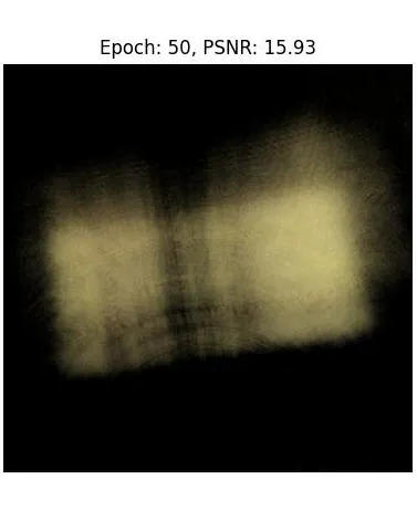
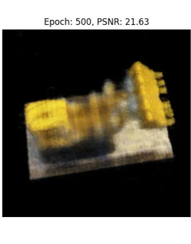
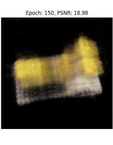
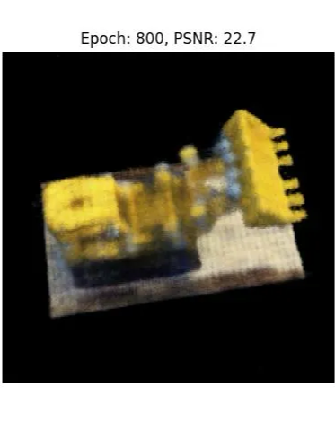
After a lot more epochs and making some of the layers deeper, we can achieve PSNRs of up to 25.3! Below

Arbitrary Camera Intrinsics to Novel View

Using the below equation for the W2C (World-to-camera) matrix, we can define a camera’s extrinsic parameters and simulate views from that camera. Specifically, we capture a camera’s position, rotation, and translation with the below expression. We can also use use the inverse of this matrix to plot points from a camera to real world points!

$$R = \begin{bmatrix} -9.4 \times 10^{-1} & -4 \times 10^{-1} & 5.3 \times 10^{-2} \\ -2.4 \times 10^{-2} & 4.2 \times 10^{-1} & -8.1 \times 10^{-1} \\ -4.5 \times 10^{-2} & -9.1 \times 10^{-1} & -5.2 \times 10^{-1} \end{bmatrix} \\ t = \begin{bmatrix} -2 \times 10^{-2}& 4.2 & 2.2 \end{bmatrix}^{\top}$$

$$W2C = \begin{bmatrix} -9.4 \times 10^{-1} & -4 \times 10^{-1} & 5.3 \times 10^{-2} & 5.3 \times 10^{-2}\\ -2.4 \times 10^{-2} & 4.2 \times 10^{-1} & -8.1 \times 10^{-1} & 4.2\\ -4.5 \times 10^{-2} & -9.1 \times 10^{-1} & -5.2 \times 10^{-1}& 2.2\\ 0 & 0&0&1 \end{bmatrix}$$

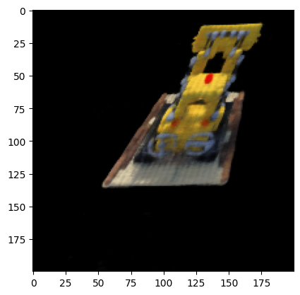
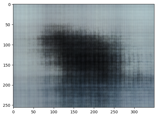
GIF Reconstruction of Novel Views from Test Set

After learning how to represent the views from the training the data, the NeRF can be tested on novel views that were never seen by the camera. In order to generate these views, we can reuse our rendering function, except we pass in a “dummy” images to compare to and feed in the extrinsic matrices that correspond to the positions and Euler angles of the new view. With this, we can ask the NeRF to return the sample along the new rays that start at these new center or projection. Then, with the Volumetric Rendering Function we can recover the estimated RGB from that pose. Below is a GIF of the test views which were never sampled for training by the NeRF. If we see any gaps in the reconstruction or artifacts that indicate a loss of volume, we can try adding more noise to the ray sampling so that the volume is implicitly “splatted,” thus preventing overfitting by the NeRF. Overfitting— in the context of NeRFs— would be the case where the NeRF learns to interpolate the pixels specifically required for the training data, possibly leaving gaps or noisy data in areas which were not sampled. As a result, our samples of novel views would have artifacts or artifacts such as pixels of incorrect colors, transparent regions, or new geometric features.

Bells and whistles:

HIGH PSNR